Sagnac, Michelson & Co
Relativity to "touch"
RuedigerRodloff
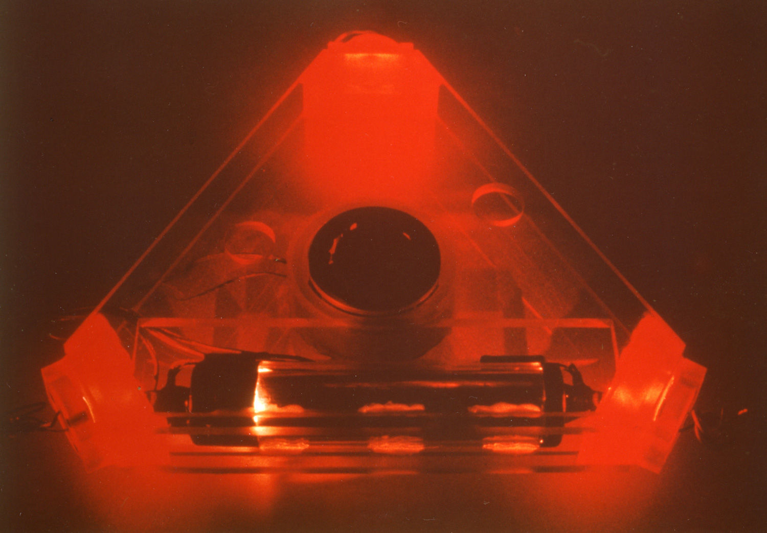
Background image - DLR - Experimental Laser Gyro - ELSY
Michelson and Sagnac as seen by Mr. Einstein
We will now finally (!) get a consistent explanation for the results of the Michelson and Sagnac experiments. We will be able to answer the question and perhaps solve the problem of whether the Sagnac is really a "purebred" relativistic effect?
First of all, we have to do some theoretical preparatory work - but don't worry - you don't need any more mathematics than before, we will only take a closer look at the directions of movement of the signal (e.g. the light wave) and the overall system (interferometer)!
Up to now we had always assumed that the direction of movement of the signal in the respective interferometer arm runs exactly parallel or perpendicular to the direction of movement of the entire system, as here in the Michelson interferometer:
Also for the annularSagnac interferometerwe assumed that the pivot point is exactly in the center of the ring-shaped light guide system, so that the movement of the light guide is always exactly parallel to the direction of movement of the light wave:

This specialization on a specific configuration is common in the literature, has made the calculation easier for us, but perhaps also blocked our view of the questions formulated at the beginning, which are of great importance for practical use as a navigation sensor.
(role of signal speed, etc.). Let's go ! How do we want to do it?
The basic idea is the following: we calculate the propagation time of a light wave in a guidance system (e.g. in an optical fiber) while the arrangement itself is moving in any other direction; e.g. as shown in the sketch here on the left!
Or to put it another way: We calculate the signal propagation time for a route element ds' and then integrate over the entire route.
We are interested in the transit time of the signal both for the way there and for the way back!
We first carry out this calculation only for a small line segment ds'. In a later step, we can then combine these path elements into a complete beam path - e.g. into a circular one as in the Sagnac interferometer. But for the clarification of some basic questions that will not be necessary at all!
We want to present the situation in a more "mathematical" way: so that we can calculate better afterwards.
The arrows (vectors) in the following sketch show the distances covered by the light wave train with the speed c' (red) and the interferometer with the speed v (black) in the time dt':
Here we use "dashed quantities" (e.g. ds', dt',...) to make it clear that we are referring to an observer who is outside the system, because it is only possible to consider the path or runtime in this situation !
(An observer moving with the measuring system can, because of the principle of relativity basically do not register a uniform movement.)

Now we have to try some trigonometry - but nothing "profound"!
The COSINE SET describes the relationship between the side lengths and the cosine of an angle in any triangle (see below) - e.g.:
c2 = a2 + b2 - 2ab cos(gamma)
or:
a2 = b2 + c2 - 2bc cos(alpha)
or:
b2 = a2 + c2 - 2ac cos (beta)

While the light wave passes through the path element ds' (red) in the time dt', the entire system (interferometer) is shifted with the speed v by the amount vdt' (black). The angle between the path element and the outer direction of movement is . Overlapping of these two movements results in resultant distance c'dt' (red dashed).
We now want to calculate the respective signal propagation times for the outward and return journeys - first for the "outward journey" (left sketch above).
According to the law of cosines, the resulting distance c'dt'hin results for the "way there".
and for the "way back":
(The relation was used !)
We will now use these relationships to calculate the signal propagation times for the outward path dt'hin and for the return path dt'back; for this we only have to solve the above quadratic equations for dt' back and forth. Here the result:

For comparison with the results from the previous chapters, we should briefly place the light wave train parallel to the external velocity v,i.e. set = 0. Then we get for the Sagnac effect:
and for the Michelson effect:
For comparison, please click: Sagnac / Michelson
In contrast to We have included previous results here to avoid confusion not on the
abbreviation resorted to, because in the
originally introduced by Einstein is with c always the vacuum speed of light cO meant.
We're actually done with that!
With these terms dt'there/back the effects for the Michelson and Sagnac interferometers can now be calculated.
The following must be considered in this regard:
In the Michelson interferometer, the light wave travels back and forth in each of the two interferometer arms. The total running time within an arm is made up of the sum of the running times dt'hin and dt'rück:
dt'Michelson = dt'there + dt'return
With the Sagnac interferometer, the two wave trains run in opposite directions through the ring interferometer and the measuring effect consists of thetransit time difference between the two waves:
dt'Sagnac = dt'there - dt'return
So - with this recipe we can now determine the runtime effects in both interferometers:

and

Well, we already knew all that!
And above all - we still have no idea why we can calculate a transit time effect for the Michelson interferometer, although it is actually not observable at all and why does it work with the Sagnac interferometer?
In order to be able to clarify this and all the other questions, we have to go one step further and bring into play the fact that with the experiments as a stationary observer we want to measure an effect in a - relative to our position - moving system.
So far we have taken the point of view of classical physics and assumed that speeds, distances and time intervals in the moving system are exactly the same as in the stationary one. As a result, we got the contradictions between reality and theory that have been discussed here several times.
So again from the beginning:
We look from the "observer system" (with primed values) onto a measuring system (with primed values) moving relative to our position with the velocity v, in which the experiment is taking place.
By the way - nobody forbids us to place the coordinate system in such a way that our further calculations become as simple as possible; I would therefore like to place the x-axes parallel to the direction of movement v of the runtime experiment:
______________
(Caution and please do not confuse - the values shown here (unlined!) refer to the measuring system moving with the speed v!)
In the last chapter of this website you will find an introduction to the special theory of relativity, where I will try to make these and similar transformations plausible (not "understandable"); until then you just have to believe me or be relevantbrowse literature!
Attention - please do not confuse: at cO is the vacuum speed of light (natural constant!) and not the signal speed c' or c - although the signal speed is identical to c in some casesO can be, we have to make a strict distinction!
We have to with all these bills Be careful as hell in which reference system we are currently: in the observer's system at rest (dashed quantities), or in the moving measurement system (undashed quantities) --> i.e. the relationships here on the right describe the path s and the angle of the light signal in (unlined) measuring system from the point of view of observer in the primed rest frame.
In this arrangement, according to Mr. Einstein, a relativistic correction must be taken into account between the moving (x,y,z) and the stationary coordinate system (x', y', z'):
with:
...all other coordinates remain as they are.
I.e. the line element ds' transforms like this:
or after some transformations:
with : --->
For the relationship between the angle in the moving system and the angle in the resting system this results in:
and with:
If we use these expressions for the line element ds' and in the above relationship for the signal propagation times dt' there/back, then we get - after "a few" transformations:
So, - done!


What have we achieved? -->As a stationary observer, we are now able to determine the signal propagation time in a moving measuring system!
Don't panic - we will use the expression for the signal propagation times in the next few sections'there/backby introducing special cases - and to keep you happy, I would like to anticipate the result of our efforts. We will show:
- there is no Michelson effect!
- the sizeof the Sagnac Effectit corresponds exactly to the classic calculation!
and very remarkable !!!
- the Sagnac effect is independent of the signal speed!
- the Sagnac effect can only be regarded as purely relativistic effect can be interpreted !